Jordan curve illustrations: attempts
The Jordan curve theorem is famously simple to state and tricky to prove. I want to explain why the Jordan curve theorem ought to be difficult to prove, by showing some pictures of very complicated Jordan curves.
This theorem states the following “obvious fact”:
Theorem (Jordan)
A simple closed curve in the plane separate the plane into two components, one bounded and one unbounded.
Here, a closed curve in the plane is a continuous map \(f: S^1 \to \mathbb{R}^2\) from a circle into the plane. It is simple when \(f\) is injective—that is, when \(f\) takes distinct points to distinct points. Simple closed curves in the plane are also called Jordan curves.
One source of such curves is simple closed approximations of space-filling curves like the one in the post on monsters:


The usual game to play with Jordan curves is to draw some horrible mess like the above, then pick a point in the middle of it off of the curve, and try to figure out if the point lies in the bounded or unbounded part. And the usual strategy for winning this game is to draw a ray starting at the given point, and to count how many times the ray intersects the curve. If it intersects the curve an even number of times, the point is in the unbounded component.
There are at least two problems with this strategy.
The first, as evidenced by the above two curves, is that there might be many intersections with the curve.
The second problem is that the strategy only works when the points of intersection of the ray and the curve are “tame,” in the sense that the local picture around the point can be isotoped to look like the intersection of two lines.
Moreover, even for the simplest possible Jordan curves, this strategy only works “generically” instead of always. The above curves show that there can be more nongeneric rays than one might want to think about. The simple picture below shows that the set of nongeneric rays can be dense for a given point.
You can get a picture like this as follows. First, recall the signum function
\[sgn(x) = \begin{cases} -1, & x < 0,\\ 0, & x = 0,\\ 1, & x > 0.\end{cases}\]Let \(\ell\) be the function of period 1 defined on \([0,1)\) by
\[\ell(x) = \frac{1+sgn(x-1/2)}{2}.\]It’s the square wave with jumps of \(-1/2\) and \(1/2\) at integers and proper half-integers, respectively, and with minimum value \(0.\)
Finally, define
\[f(x) = \sum_{i \geq 1} 2^{-i} \sum_{0 \leq j < 2^{i-1}} \ell\left(x-\frac{2j+1}{2^i}\right).\]Or, if you like, for \(x \in [0,1)\) we define \(f(x) = \int_0^x d\mu,\) where \(\mu\) is the measure with a point mass at \((2j+1)/2^i\) of weight \(1/2^i\) for all such dyadic rationals in \([0,1).\)
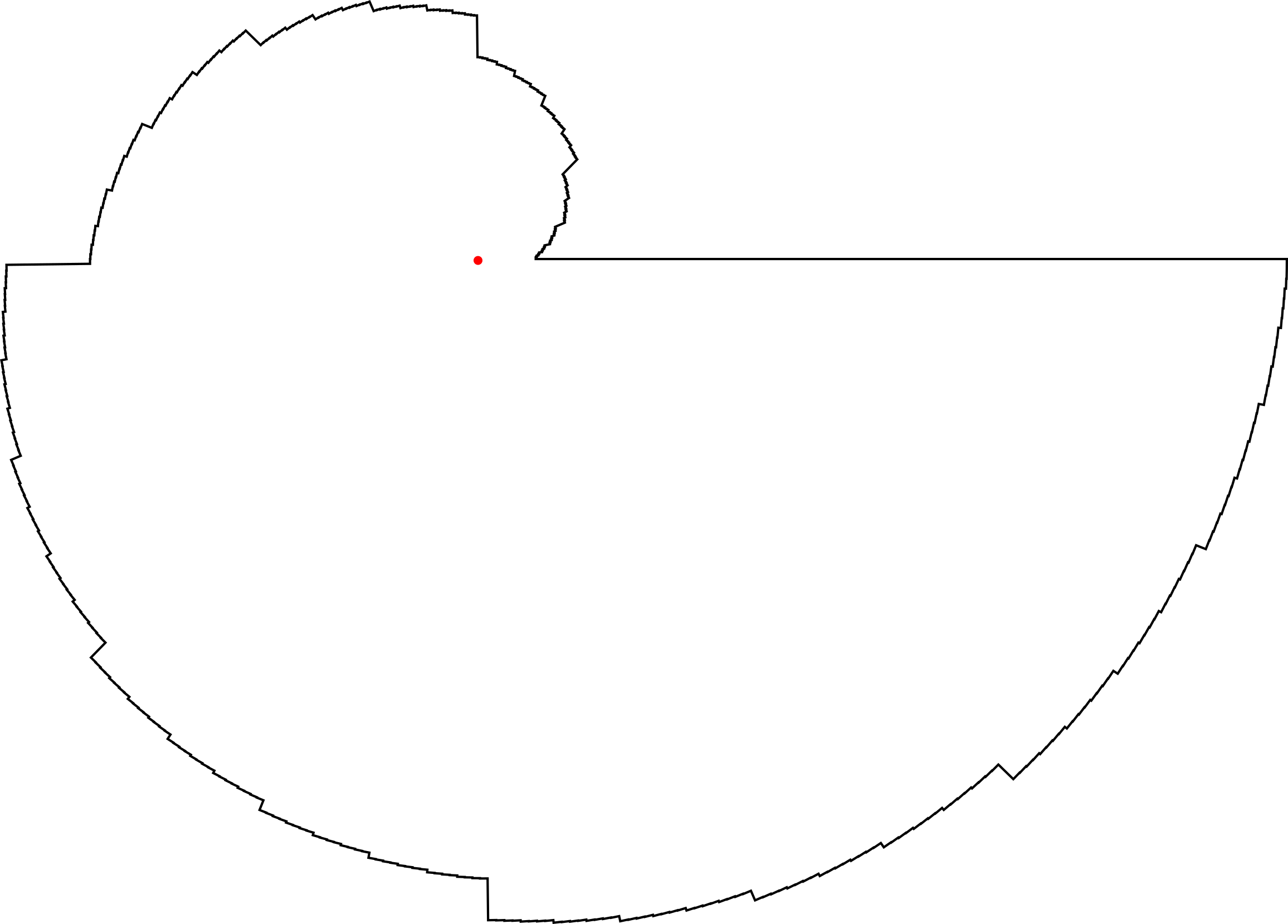
Then the graph of \(f\) has a jump discontinuity at every dyadic rational. This remains true when we draw the graph of \(r = 1+f(\theta/(2\pi))\) in polar coordinates. Plugging the jumps with segments yields a Jordan curve like the one above. Every ray from the origin at a dyadic fraction of a full turn intersects this curve in a segment of positive length, and the set of such rays is dense.
These curves should give the reader pause. But in my opinion, they are not sufficiently representative examples. For instance, in the previous example one can draw from the red dot a small segment downwards, and then draw a segment going northeast and intersecting the curve in its longest segment. So, even though there is no ray from the red dot intersecting the curve nicely, there is at least a (fairly easy-to-spot) piecewise-linear path from the red dot that intersects the curve nicely. Moreover, the first examples, although very complicated, do not limit on an “infinitely complicated” curve. Instead, they limit on a square, which is certainly1 not a single curve. This raises the question of whether there is a Jordan curve \(\Gamma\) such that every piecewise-linear path from the bounded component to the unbounded component intersects \(\Gamma\) infinitely many times. This would be representative of the complicated, awkward nature of “generic” Jordan curves. Constructing and drawing a well-motivated2 such curve is the subject of the next few posts.
Footnotes
-
I say “certainly,” but this is also not particularly easy to prove. It comes from what’s called invariance of domain. ↩
-
One can construct such curves as the limit sets of quasi-Fuchsian Kleinian groups, e.g., this image of Jos Leys (images 42, 44, 45b–d, 49, 52, 53, 59, and 68 from the same gallery are also good examples). These are certainly important objects, but their motivation would take us far afield. ↩