Jordan curve illustrations: drawing the curve
There is a Jordan curve such that every piecewise-linear path from the inside to the outside intersects the curve infinitely many times. I describe how to draw such a curve here, and do so.
Generating a point sequence
It is easiest to describe wiggling as in the previous post. One could encode courses directly using turtle graphics. However, the number of segments to draw in the final picture is quite large. Suppose we begin with a simplest hex loop, with course \(PPPPPP.\) Every wiggling multiplies the number of tokens by \(49.\) After just three wigglings the number of segments is \(705894.\) We intend to draw the resulting hex curve. To use turtle graphics would mean to use floating point arithmetic to accomplish rotations by 120 degrees port or starboard. After so many rotations and additions, it is reasonable to suspect the resulting “curve” wouldn’t close up. On the other hand, no triple of points in the grid of integers forms an equilateral triangle. So what we do is work over the integer lattice when calculating a point sequence directly from a course. Then after all those points are determined, we apply an affine equivalence from the square grid lattice to the penny-packing lattice. This will give us a closed hex curve, as a sequence of points we may feed to PostScript.
To fix ideas, begin with the lattice \(\Lambda^3\) generated by \(v_s = (1,0)\) and \(v_p = (-1/2,\sqrt{3}/2).\) We label these vectors so because if a hex curve comes into a vertex at \(vtx = (0,0)\) from \((-1/2, -\sqrt{3}/2)\) along the incoming vector \(v_i = v_s + v_p,\) then a starboard turn at \((0,0)\) would go along \(v_s,\) whereas a port turn at \((0,0)\) would go along \(v_p.\)
In general, at a vertex \(vtx\) a hex curve has an incoming vector \(v_i\) that is the sum of the outgoing port and starboard vectors \(v_p, v_s.\) More specifically, letting \(\rho\) be counterclockwise rotation by \(2\pi/3,\) we have \(v_s = \rho(-v_i)\) and \(v_p = \rho(v_s).\)
Suppose a hex curve takes a starboard turn at \(vtx.\) Then:
- the next vertex position would be at \(vtx + v_s;\)
- the next incoming vector would be the current \(v_s;\)
- the next starboard vector would be \(\rho(-v_s) = -v_p;\) and
- the next port vector would be \(\rho(-v_p) = v_i.\)
If a hex curve takes a port turn at \(vtx\) instead, then:
- the next vertex position would be at \(vtx + v_p;\)
- the next incoming vector would be the current \(v_p;\)
- the next starboard vector would be \(\rho(-v_p) = v_i;\) and
- the next port vector would be \(\rho(v_i) = -v_s.\)
That is, a starboard turn accomplishes the state change
\[(vtx,v_s,v_p,v_i)\ \leftarrow\ (vtx+v_s,-v_p,v_i,v_s),\]whereas a port turn instead accomplishes
\[(vtx,v_s,v_p,v_i)\ \leftarrow\ (vtx+v_p,v_i,-v_s,v_p).\]To convert a course of turn-type movement tokens into a sequence of points, then, we begin with an appropriate initial collection of incoming, port, and starboard vectors, and some initial vertex, and we simply apply the appropriate state changes above according to the sequence of tokens, keeping track of the points seen in order. We may encode this in Python as follows:
def add(v,w):
    return (v[0]+w[0],v[1]+w[1])

def negate(v):
    return (-v[0],-v[1])

def to_points(course, start):
    vtx,vs,vp,vi = start
    points = [vtx]
    toks = list(course)
    toks.reverse()
    while len(toks) != 0:
        tok = toks.pop()
        if tok == 'S':
            vtx,vs,vp,vi = add(vtx,vs),negate(vp),vi,vs
        elif tok == 'P':
            vtx,vs,vp,vi = add(vtx,vp),vi,negate(vs),vp
        else:
            raise Exception("Bad token")
        points.append(vtx)
    return points
N.B. the tokens are reversed in to_points because Python pops elements from the end of a list, not the beginning.
Drawing the curve
We could choose a different lattice \(\Lambda = \langle v_s, v_p \rangle\) and still run the above code (starting with \(vtx = (0,0),\) say). The resulting points are the vertices of a PL curve affinely equivalent to the desired sequence in \(\Lambda^3,\) via the unique linear map \(v_s,v_p \mapsto v_s^3,v_p^3.\) Another way to look at this is that we generate first the (integer) coordinates of the points with respect to the basis \((v_s^3, v_p^3),\) then determine their Cartesian coordinates.
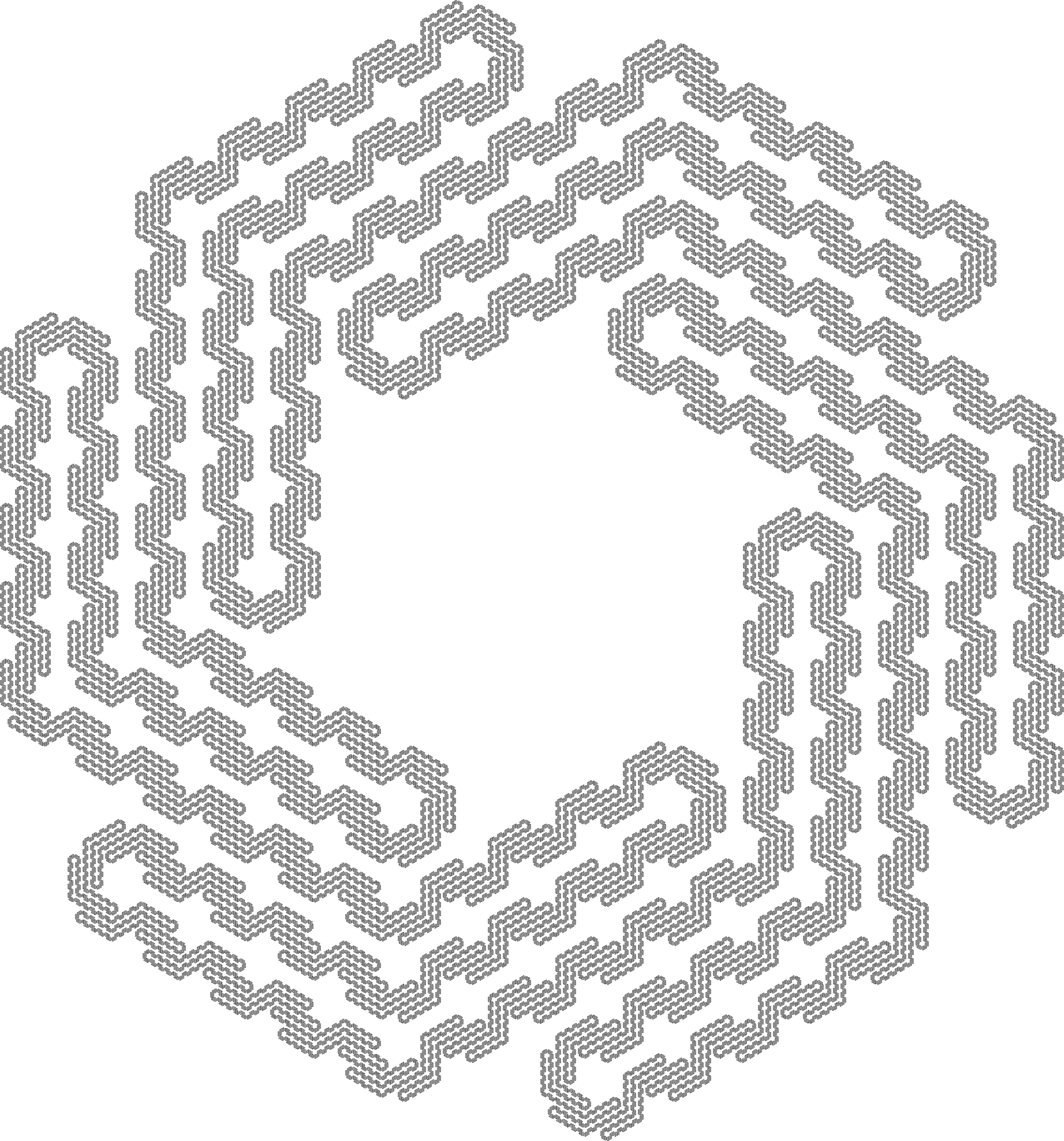
Finally, we would like all this to fit on a U.S. letter page. This is not difficult to organize. So, the following code, together with the code above, generates a PostScript file of the third wiggling of the simplest hex loop “PPPPPP,” illustrating what the limit Jordan curve looks like.
def draw(pts):
    with open("jordan.ps",'w') as ps:
        (x0,y0) = pts[0]
        minx,maxx,miny,maxy = x0,x0,y0,y0
        for (x,y) in pts[1:]:
            minx,maxx = min(minx,x),max(maxx,x)
            miny,maxy = min(miny,y),max(maxy,y)
        midx = maxx//2+minx//2+(maxx%2+minx%2)//2
        midy = maxy//2+miny//2+(maxy%2+miny%2)//2
        rngx = maxx-minx
        rngy = maxy-miny

        ps.write("%!\n")

        # Fit US Letter size page to curve
        ps.write("72 dup scale\n") # Length in inches
        ps.write("{0} {1} translate\n".format(8.5/2,11/2))
        scale = min(8.5/rngx,11/rngy)
        ps.write("{0} dup scale\n".format(scale)) # Length in coords
        ps.write(".95 dup scale\n") # Margin room

        # Draw curve
        ps.write("newpath\n")
        ps.write("{0} {1} moveto\n".format(x0-midx,y0-midy))
        for (x,y) in pts[1:]:
            ps.write("{0} {1} lineto\n".format(x-midx,y-midy))
        ps.write(".111 setlinewidth\nstroke\n")
        ps.write("showpage\n")
        ps.close()

from math import sqrt

if __name__ == "__main__":
    simple = "PPPPPP"
    intpts = to_points(wiggle(wiggle(wiggle(simple))))
    s32 = sqrt(3)/2
    hexpts = [(x-0.5*y,s32*y) for (x,y) in intpts]
    draw(hexpts)
The ensuing PostScript file is rather large; I converted it to PDF and thence to a PNG file. Here is what it looks like:
That is the construction. It remains to be shown that it has the two desired properties, namely
- that its limit yields a Jordan curve; and
- that Jordan curve intersects no PL curve in a positive finite number of points.
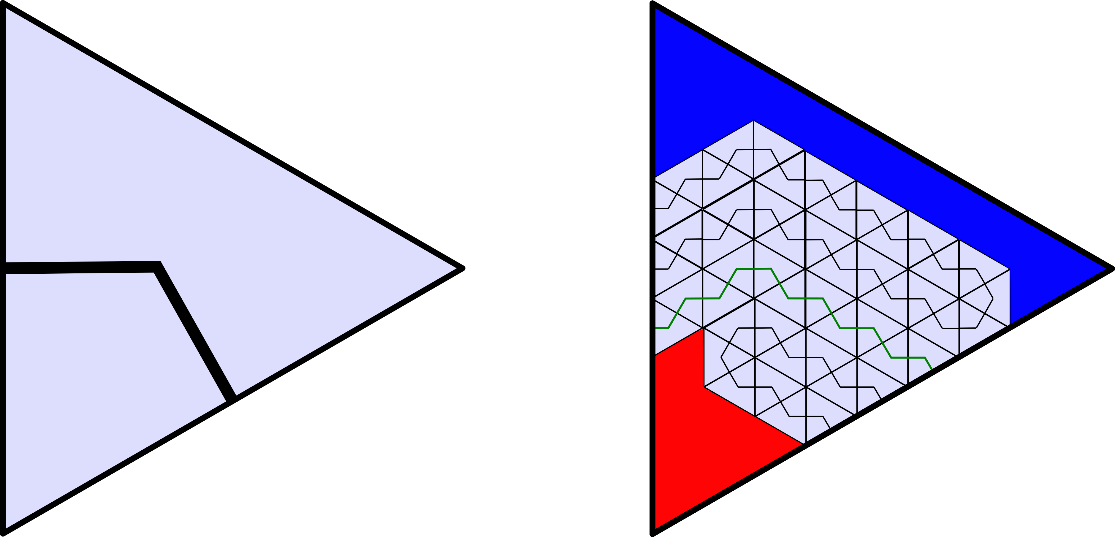
Roughly speaking, here are why these properties hold. This yields a Jordan curve because we leave enough space in the triangles so that the curves limit on an continuous injection, and because a point in a triangle of the curve is only wiggled to “nearby” triangles. The Jordan curve is crossed finitely by no PL path because in each triangle, every line segment between the blue and red regions from the first triangle post crosses the curve more than once.
That “explanation” is what G. H. Hardy would call gas. But it’s all I’m putting down for right now!