Jordan curve illustrations: idea for a better example
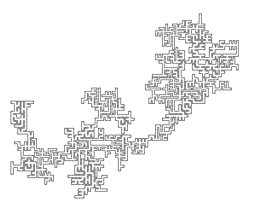
There is a Jordan curve such that every piecewise-linear path from the inside to the outside intersects the curve infinitely many times. We will begin the construction of such a curve here.
The construction is inspired by this sketch on MathOverflow by Anton Petrunin. The basic idea is to keep wobbling a curve locally at ever smaller scales. Of course, it is very important how and at what scales one wobbles; otherwise one might end up with, for instance, the square-filling pictures from the last post. So let’s fix some definitions and refine the basic idea.
First, we will choose an explicit class of curve to draw. The simplest interesting curves are the rectagons.1
Definition:
A simple closed curve \(\gamma: S^1 \to \mathbb{R}^2\) is a rectagon when its image is the union of finitely many horizontal and vertical unit line segments with endpoints in \(\mathbb{Z}^2.\)
However, a Jordan curve limit of rectagons will just be another rectagon. To get the desired limit we will employ appropriately scaled rectagons:
Definition:
A simple closed curve \(\gamma: S^1 \to \mathbb{R}^2\) is digital when it is the image of a rectagon under a scaling map \((x,y) \mapsto (2^{-n} x, 2^{-n} y)\) for some \(n \in \mathbb{N}.\)
Equivalently, a digital curve is a rectagon whose image is the union of finitely many horizontal and vertical line segments with endpoints in \(\mathscr{B} = \mathbb{Z}[1/2]^2,\) the collection of points in the plane whose coordinates have finite binary place-value expansions, hence the name digital.
We will construct the desired Jordan curve as a limit of digital curves. To that end, let us establish explicit representations of digital curves. One obvious such representation is as sequences of points
\[(0,0), (x_0, 0), (x_0, y_0), \ldots, (x_i, y_i), (x_{i+1}, y_i), (x_{i+1}, y_{i+1}), \ldots, (x_n, y_n), (0, y_n), (0,0)\]where one coordinate changes between consecutive points, and where for all \(i,\) \(x_i \in \mathscr{B}.\) This is useful for proving the Jordan curve theorem for digital curves.
Here is another way to represent a digital curve that is more convenient for our purposes. A digital curve is a rectagon \(\gamma\) scaled by some factor \(2^{-n}.\) For every point \((x,y) \in \mathbb{Z}^2\) on \(\gamma,\) consider the intersection of \(\gamma\) with the unit square \([x-1/2,x+1/2]\times[y-1/2,y+1/2].\) Orienting \(\gamma,\) up to rotational symmetry there are only three nonempty types of intersection: Forward, Left, and Right.

Thus \(\gamma\) may be represented as a sequence of movement tokens
\[n_0\, A_0\, n_1\, A_1 \ldots,\]where each \(A_i\) is either Left or Right, and where a natural number indicates that number of Forward intersections. This sequence together with the scaling factor \(2^{-n}\) we will call the intrinsic representation of the associated digital curve.2
Our goal is to wiggle, i.e. isotope, the curve on smaller and smaller scales, but not so much that it is no longer a curve. I’ll try to articulate the motivation for this construction now. First, once we multiply by the factor, scaled unit squares could constitute good local pictures at smaller and smaller scales. We want to isotope the local pictures in these squares in such a way that digital segments from one side of the arc to the other in the square must intersect the arc in multiple points. To be more precise, in each of the above pictures, the arc cuts the square into two pieces, say Port and Starboard. After isotopy, we want all digital segments from the Port parts of the square’s boundary to the Starboard parts to intersect the arc multiple times.
Now, the most obvious such digital segments are the sides of the square perpendicular to the arc. After isotopy, these need to intersect the arc multiple times. Now, if we’re just going to wiggle the arc a little bit, then we can only introduce an even number of additional intersections of the arc with these sides. For a simplest possible picture then, we want to have three intersection points with the incident sides. However, we cannot simply replace the given arc with three parallel arcs; that would create two new curves. After some trial-and-error,3 you could come up with the following pictures as I did:


If we isotope the green rectagon in the left squares as shown above, we get a digital curve that is a rectagon scaled by \(2^{-3}.\) One would like to say that the new rectagon is just the old rectagon, but with Forward tokens replaced with a new sequence of tokens, and likewise for Left and Right tokens. This is technically true, but is misleading, since the replacements depend not only on the tokens, but also on their neighbors. I will show how I organized this in the next post.
Footnotes
-
This terminology is from Hales’s Monthly article on formally proving the Jordan curve theorem. ↩
-
Après Logo, we might also call this the turtle representation. ↩
-
Or after thinking about thin position. ↩